 |
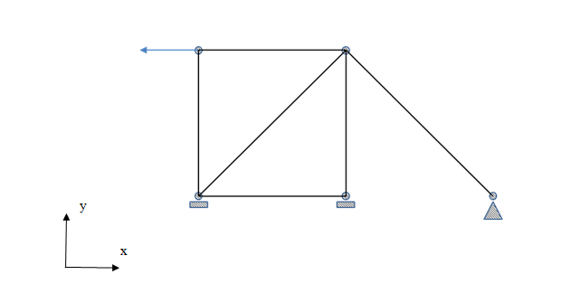
Part 1 - Introduction - Direct Stiffness methods:The direct stiffness method is a classical method that uses matrices to solve structural problems. The method enables a systematic approach that is scalable, enabling solutions to many kinds of problems. Consider the following statically indeterminate situation:
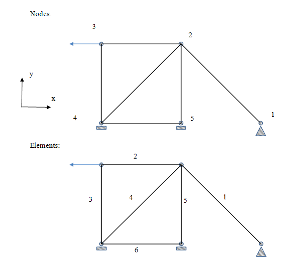
Good engineering practice always involves some kind of simplifying assumption, idealization, or judgment. The following beam structure above is statically indeterminate, so one approach to solve the problem as a function of applied loads and model configuration (stiffness matrix), is the direct stiffness method. This matrix method breaks the problem down into members and connecting points (elements and nodes) where a direct stiffness formulation is known. Then building on that, a global stiffness matrix can be built up based on the individual element connectivity. Using a computer, this method, once programmed can easily be applied to compute structural solutions to various problems. Part 02 - Getting StartedLet's get started. First we will have to assign node and element numbering to the model so it is always clear what details we are currently discussing. Consider the following numbering:
For example to element 1 goes between node 1 and node 2.
In order to solve for loads, reactions, and stresses the model needs some basic definitions. For example what the elements are shaped like, what kind of material are they made of and what are the dimensions of this model. Let's assume the members have a cross section of an I-Beam one inch high, 0.25" wide with a flange thickness of 0.050". This results in a cross section area of: 0.07" and a moment of inertia of 8.683E-03. Additionally let's say the sections are aluminum (Young's Modulus, E, of 10.3E6 psi). Now all that remains of problem definition is the magnitude of the load (say 100 lbs), and node coordinates to establish the length of the elements.
The last component of the model is the "constraint set". As indicated in the graphic this has already been established, nodes 1, 4 and 5 are constrained. 4 and 5 are "fixed" and can resist vertical, horizontal loads and moments. What this means, is that as the structure deforms under the applied load they can not move, nor can they rotate (no translation, no rotation). Node 1, however only has a translation constraint (a pinned connection) and is free to rotate. This establishes the base model information and we can begin the solution. The basic direct stiffness method establishes a local stiffness matrix for each element in its local coordinate system. This is important because no matter the connectivity or orientation of the element the formulation is the same. This allows the model to be simplified and hence processed in a very uniform way.
Part 03 - Local Element Stiffness Formulation
The element local stiffness matrix is a function of the element length, Young's modulus, and moment of inertia. Often called frame, truss or beam elements for this problem we will use elements that can transmit forces in tension, compression and bending. This three degree of freedom (x, y, and theta) results in a 6 x 6 stiffness matrix for each element. Before establishing the 6x6 it is important to first review the method in 1 DOF (degree of freedom). Take for example a simple 1 DOF spring: where: f=k*x This is part of the beauty of matrices, as they are readily scalable. This same formulation can be used for the 3 DOF problem at hand, locally, and then expanded into a global stiffness matrix to solve the original problem. The general stiffness matrix "k" from above is:
For the element type chosen this becomes:
This local stiffness matrix can easily be calculated for each element in its local coordinate system as a function of some basic elemental parameters (properties). For example: Element 4: A = 0.07 in2 E = 10.3e6 psi I = 8.683E-03 in4 Determining the element length is a simple matter of calculating the distance between its nodes (node 2 and node 4).
Calculating the element length: \begin{align} L & = \sqrt{(x_4-x_2)^2+(y_4-y_2)^2}\\ L & = \sqrt{(0-10)^2+(0-10)^2}\\ L & = 14.142\\ \end{align} This results in a local matrix of:
Part 04 - Local to Global Element Stiffness Formulation
With the local stiffness matrix evaluated this needs to be put within the context of the global problem. Remember where this element was situated in the structure configuration (between nodes 2 & 4):
Let's say that the element goes from node 4 to node 2. This would allow us to develop a rotation to translate the local formulation into a relative global configuration. We can determine this rotation from the nodal coordinates. Using trigonometric relations between the nodes the rotation matrix into global:
\begin{align} \frac{x_4-x_2 }{ L }\\ \frac{y_4-y_2 }{ L }\\ \end{align}
Evaluating the matrix:
Applying this rotation mayrix to the local stiffness matrix will result in a global stiffness matrix for this element, in the global coordinate system. The result of this application is:
With this established there are four sub quadrants identified in the stiffness matrix, each consisting of 9 values. It may be simplest to think of them as contributions to the global stiffness from various perspectives. Looking at the upper left quadrant:
Let's call this node 2's local effect, IE node 2 looking toward node 2. Next the upper right:
Let's call this stiffness at node 2 looking toward node 4. Next the lower left:
Let's call this stiffness at node 4 looking toward node 2. Finally, Looking at the lower right quadrant:
Let's call this node 4's local effect, IE node 4 looking toward node 4. . This procedure is completed for each element in the system. So you can check your work, here are the global contributions for each element in this system.
Part 05 - Assembly of Global Matrix
Now each of the individual global stiffness matrices need to be combined into one matrix to solve the problem. Each matrix on its own is in global coordinates, however it does not take into account how it is positioned to the other elements in the model. To do this a stiffness matrix of (sum(#of nodes*DOF)) x sum((# of nodes*DOF)) needs to be created. For this problem that is simply (5 nodes * 3 DOF) or a 15*15 matrix. Remember the three degrees of freedom in this problem are: x, y, & theta (x translation, y translation, and rotation)
Think of the global stiffness matrix as positioning yourself at one node and looking at the stiffness contributions at each of the other nodes in each of the degrees of freedom. Positioning ourselves at node 1 we will look in each DOF at each node (including the local stiffness where we are, so at node 1 looking at node 1).
Remember the model configuration:
Node one is relatively easy because it does not have multiple connectivity, it only has element 1 that connects to it and leads to node 2. This can be contrasted at node 2 which has connectivity to nodes 1,3, & 5 via elements 1, 2, and 5 respectively. Back to node 1: Summing all elements sub matrices of at node 1, looking to node 1 (there is only one contributor element 1):
sum of node 1 looking to 2 (there is only one contributor element 1)
sum of node 1 looking to 3, 4, and 5 there are no contributions from any elements and these values are all zero.
moving to node 2 now: Summing all elements sub matrices of at node 2, looking to node 2 (there are four contributors elements 1,2,4,5):
Element 1 node 2 looking toward node 2:
Element 2 node 2 looking toward node 2:
Element 4 node 2 looking toward node 2:
Element 5 node 2 looking toward node 2:
The sum of these results in the global stiffness sub matrix of node 2 looking towards node 2:
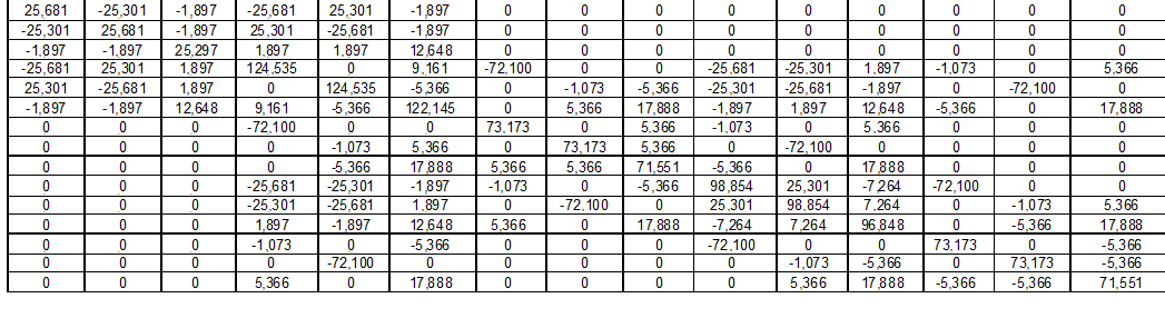
Using this method of positioning at each node and summing the stiffness contributors to each of the other nodes the following 15 x 15 matrix is constructed.
Part 06 - Constraints & Loads - Reduced Global Stiffness Matrix
This global matrix represents numerically the structure. It does not take into account the constraint or load configuration. Going back the f=kx the constraints are first applied.
In this problem the DOF of each node if constrained is noted as follows:
What this means is that: Node 1 can is restricted from any movement in the x & y directions. Node 4 can is restricted from any movement in the x & y directions, and is restricted from any rotation. and Node 5 can is restricted from any movement in the x & y directions, and is restricted from any rotation. Taking these constraints into account enables the creation of a reduced stiffness matrix. To do this the rows and columns that correspond with the constrained degrees of freedom are simply deleted from the global stiffness matrix. This means rows and columns 1,2, & 10-15 are removed. To illustrate this more clearly, the following figure shows which rows / columns are deleted:
This reduced stiffness matrix resulting is as follows:
This is when we can now go back to the F=kx formulation again. For this problem the F matrix only has one applied load and hence has the formulation of:
Deleting the same rows as with the stiffness matrix leaves:
X can now be solved for by multiplying F and the inverse reduced stiffness matrix. (f*k-1=x) This results is the following nodal deformations:
We now have a complete set of nodal deformations as follows:
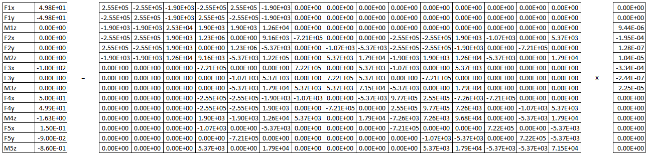
With the global stiffness matrix and the global deflections known, all the forces can now be solved for again using the f=kx formulation.
Re-formatting the force matrix we find the external constraint forces:
* as a check the sum of the forces in each direction always need to equal zero. If it does not this implies static equilibrium is not maintained. Modeling the problem in FEMAP & NX NASTRAN shows good results correlation:
|
|||||||||||||||||||||||||||||||||||||||||||||||||||||||||||||||||||||||||||||||||||||||||||||||||||||||||||||||||||||||||||||||||||||||||||||||||||||||||||||||||||||||||||||||||||||||||||||||||||||||||||||||||||||||||||||||||||||||||||||||||||||||||||||||||||||||||||||||||||||||||||||||||||||||||||||||||||||||||||||||||||||||||||||||||||||||||||||||||||||||||||||||||||||||||||||||||||||||||||||||||||||||||||||||||||||||||||||||||||||||||||||||||||||||||||||||||||||||||||||||||||||||||||||||||||||||||||||||||||||||||||||||||||||||||||||||||||||||||||||||||||||||||||||||||||||||||||||||||||||||||||||||||||||||||||||||||||||||||||||||||||||||||||||||||||||||||||||||||||||||||||||||||||||||